Google Sheets tutorial
How to make a graph in Google Sheets
 SayScreen
This whole video was made by AI.
Make your own at sayscreen.com
$1 for 7 days, then $49/month
- 2:27 video
- 8 steps
- Last verified November 13, 2026
A graph in Google Sheets starts with your data in columns: labels in the first, numbers in the next. This video types six months of sales, selects them and inserts a chart, which opens the Chart editor. It tries a column chart, then a line chart to show the trend, titles it Sales by Month on the Customize tab and drags it beside the data.
Steps
- Type the data in two columnsMonth in A1 and Sales in B1, then January to June in A2:A7 and their sales in B2:B7: 1200, 1500, 1350, 1800, 2100 and 2400.
- Drag from A1 to B7 to select itInclude the headers: Sheets uses them to label the chart.
- Open Insert and choose ChartSheets builds a chart from your selection right away and opens the Chart editor on the right.
- Choose Column chart under Chart typeOn the Setup tab, open the Chart type list. A column chart compares amounts side by side, like sales in each month.
- Switch to Line chartOpen the list again and choose Line chart to show the trend over time.
- On the Customize tab, title it Sales by MonthExpand Chart & axis titles. With Chart title selected, replace the Title text.
- Drag the chart beside the dataThe new chart covers part of the table, so drag it to the right.
- Close the Chart editorThe finished line chart sits beside the table. Double-click it to open the editor again.
Transcript
0:00In this video, you'll learn how to turn a simple table of numbers into a graph in Google Sheets. We'll start with an empty spreadsheet.
0:09First, the data. In cell A1, type the header Month. Below it, list the months January through June, pressing Enter after each one to move down a row. In column B, add the header Sales, then each month's figure: twelve hundred, fifteen hundred, thirteen fifty, eighteen hundred, twenty-one hundred, and twenty-four hundred.
0:43Next, tell Sheets which data to chart. Drag from A1 down to B7 so both the headers and the numbers are selected.
0:53With the range selected, open the Insert menu. Choose Chart, and Sheets builds one from your selection right away. The chart editor opens on the right. On the Setup tab, you control the chart type, the data range, and which columns feed the axes.
1:11Open the Chart type dropdown to see every style of chart available. Pick Column chart. Column charts are great for comparing amounts side by side, like sales in each month.
1:24To show the trend over time instead, open the dropdown again. This time choose Line chart. A line connects the months, making the steady climb in sales easy to see.
1:37Now give it a clearer title. Switch to the Customize tab, where you style every part of the chart. Expand Chart and axis titles. With Chart title selected, replace the title text with Sales by Month.
1:56The chart is covering part of the table, so drag it to the right and drop it beside the data.
2:03Close the chart editor to see the finished result. And that's it: you entered your data, inserted a chart, tried column and line styles, gave it a title, and placed it right beside your table.
Google Sheets is a trademark of its owner. SayScreen isn't affiliated with, sponsored or endorsed by Google Sheets; this video shows the public app as it looked when it was recorded, and we last checked the steps on November 13, 2026. If Google Sheets has changed since, tell us at hey@sayscreen.com. Google Sheets's own guide: support.google.com/docs/answer/63824.
More how-to videos
All Google Sheets videos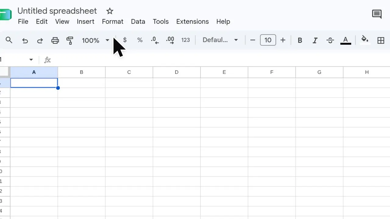 4:02Google SheetsHow to make a Gantt chart in Google Sheets11 steps · Verified November 6, 2026
 4:02Google SheetsHow to create a dropdown list from another tab in Google Sheets10 steps · Verified November 6, 2026
 2:51Google SlidesHow to add a video to Google Slides11 steps · Verified November 13, 2026